


2. 华东师范大学城市与区域科学学院, 上海 200241;
3. 西南交通大学地球科学与环境工程学院, 四川 成都 611756;
4. 北京师范大学地表过程与资源生态国家重点实验室, 北京 100875
2. School of Urban and Regional Science, East China Normal University, Shanghai 200241, China;
3. Faculty of Geosciences & Environmental Engineering, Southwest Jiaotong University, Chengdu 611756, China;
4. State Key Laboratory of Earth Surface Processes and Resource Ecology, Beijing Normal University, Beijing 100875, China
高光谱图像已被广泛用于地质、生态、大气、医学、农业等领域[1-2]。其波段数目众多且相邻波段相关性较高,需进行降维处理[3]。常见的高光谱数据降维处理方法有考虑所有波段的数学变换方法及波段组合方法[4]。前者过程复杂、计算量大,且改变了高光谱图像的物理意义。后者更为常用,包括监督和非监督两类[5]。
非监督波段选择多基于波段排序和聚类[6]。波段排序方法例如信息离散度法(information divergence,ID)[7]、线性约束最小方差法(linearly constraint minimum variance,LCMV)[8]和最大方差主成分分析法(maximum variance principal component analysis,MVPCA)[7]。这些方法虽然直观简便,但忽略了波段间相关性,导致冗余波段。波段聚类先将相关性强的波段聚成一组,再挑选各组的代表性波段。聚类多基于互信息(Ward's linkage strategy using mutual information,WaLuMI) 和KL散度(Ward's linkage strategy using divergence,WaLuDi)[9]。人工智能也被用于波段聚类与选择,如文献[10]基于深度学习对高光谱数据降维处理。文献[11]结合深度卷积自编码器和子空间聚类进行波段选择。文献[12]采用深度对抗子空间聚类(deep adversarial subspace clustering,DASC)网络以提升子空间聚类的自表达能力,文献[13]基于全连接深度网络和深度神经网络提取波段间的非线性特征。
最优波段组合为信息丰富且各波段间的相关性最小的波段集合[14]。作为传统信息测度指标,香农熵仅考虑了空间组分信息(像元的种类和比例)[15-17],忽略了空间配置信息(像元的空间分布),无法准确刻画图像相似性[18]。如图 1所示,图 1(a)与1(b)的组分不同、但配置相同;图 1(a)与1(c)的组分相同、但配置不同。

|
| 图 1 具有相同组分或配置信息的不同图像 Fig. 1 Different images with the same composition or configuration information |
香农熵因热力学基础薄弱、忽略了空间配置信息等受到质疑[16]。玻尔兹曼熵(简称玻熵)被引入以克服上述不足,包括基于边缘总数的玻熵[19]、基于多尺度层次结构的玻熵[20]等。文献[21]提出了基于Wasserstein指标的配置熵(简称W熵)测度指标,本文将其引入高光谱图像波段选择,将W熵从四邻域拓展至八邻域。基于W熵差异值测度高光谱图像波段间的相关性,通过非监督次优搜索法确定最优波段组合,使用支持向量机(support vector machine, SVM)分类,评价其分类精度。
1 空间信息与相关性测度当前测度波段信息和波段相关性主要有两类方法,即香农熵和玻熵。
1.1 空间组分信息:从香农统计信息熵到香农空间信息熵信息是"事物运动状态或存在方式的不确定性"[15],信息量是对信息统计特征的描述,公式为
 (1)
(1)
式中,P(x)表示随机变量X取值为x的概率。
文献[22]构建了地图符号多样性信息熵测度指标。文献[17]指出地图信息包括统计、几何、拓扑和专题信息等,提出基于Voronoi图的信息熵计算方法,是现有对地图信息的最佳量测[15]。文献[23]构建了香农熵变体。
1.2 空间配置信息:玻尔兹曼熵玻熵源于热力学[24],公式为
 (2)
(2)
式中,S为某宏观状态的玻熵;kB为玻尔兹曼常数;W为该宏观状态中所包含的微观状态总数。W熵是玻熵的变体,基于Wasserstein距离构建,即两个概率分布之间转换的最小代价[25],公式为
 (3)
(3)
式中,(Pr, Pg)是边缘分布Pr和Pg的联合分布;∏(Pr, Pg)是联合分布(Pr, Pg)的集合。W熵指标[21]公式为
 (4)
(4)
式中,Wc和Ws分别为改进版玻熵计算公式中第2项对应的直方图、第3项对应的直方图与狄拉克分布变体之间的Wasserstein距离的归一化结果。
图 2(a)尺寸为512×512像素,分别取其灰度矩阵的前128、256、384及512列像元灰度值进行随机排列,得到图 2(b)至图 2(e)。图 2(a)至图 2(e)的W熵分别为0.422 0、0.422 4、0.423 0、0.424 5和0.426 6,与目视观察到的无序性程度一致,表明W熵可刻画图像空间配置复杂性。

|
| 图 2 某图像及部分像元随机排列后的图像 Fig. 2 A image and its randomly permuted images |
1.3 信息的相关性:互信息、相对熵与玻熵差异值
两个随机变量的相关性可由互信息或相对熵测度。
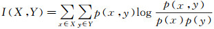
1.3.1 互信息互信息描述了两个随机变量之间的统计相关性,即某随机变量包含另一随机变量信息的不确定性程度,公式为
 (5)
(5)
式中,p(x, y)是两个随机变量X、Y的联合概率分布函数;p(x)和p(y)分别是随机变量X、Y的边缘概率分布函数。变量相关性越强,包含的共同信息越多,互信息值越高。互信息具有对称性。
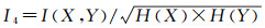
1.3.2 标准化互信息因变量类型与取值范围的差异,对互信息进行标准化处理[26-27],包括
 (6)
(6)
 (7)
(7)
 (8)
(8)
 (9)
(9)
式中,I(X, Y)是两个随机变量X和Y的互信息;H(X)和H(Y)为X和Y的香农熵。
1.3.3 相对熵相对熵(又称为KL散度)是两个概率分布差异的非对称性测度[28],公式为
 (10)
(10)
式中,P(X)和Q(X)分别为随机变量X的两种概率分布。
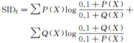
1.3.4 相对熵变体为避免Q(X)=0,文献[9]提出两个应用范围更广的相对熵变体
 (11)
(11)
 (12)
(12)
式中,P(X)和Q(X)分别是随机变量X的概率分布。
表 1列出图 2中影像两两间相似性计算结果,证实了互信息和标准化互信息的有效性。
1.3.5 玻熵差异值
绝对或相对玻熵差异值也可刻画波段相似性[9],公式如下
 (13)
(13)
 (14)
(14)
式中,X和Y代表不同波段;SA和SR代表绝对和相对玻熵。
W熵差异值公式为
 (15)
(15)
式中,X和Y代表不同波段;W代表各波段的W熵。
2 Wasserstein配置熵的改进及其用于波段选择的基本思路传统W熵局限于四邻域,本文将其拓展到八邻域,并提出基于W熵的高光谱图像波段选择方法。
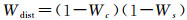
2.1 W熵的改进:从四邻域到八邻域邻域广泛见于斑块镶嵌体格局、地理相似性或空间自相关分析中[29]。常见的邻域定义方式有Rook(仅共边)邻近、Bishops(仅共顶点)邻近和Queen's(或King's)(共边或共顶点)邻近[30]。前二者为四邻域,后者为八邻域,对应的W熵分别记为Wdist和W8dist。
图 3中,各影像对应的Wdist值分别为1.000 0、0.955 3、0.977 4和0.977 4,对应的W8dist值分别为1.000 0、0.955 3、0.955 3和0.977 4。表明W8dist可有效识别连续区域引起的信息冗余。

|
| 图 3 4幅模拟图像 Fig. 3 Four simulated images |
2.2 基于W熵的波段选择思路
采用文献[5]提出的非监督次优搜索法来确定信息量较大且相关性较低的波段组合。具体过程如图 4所示,其中α和β分别代表原始波段集合和最优波段集合。

|
| 图 4 基于Wasserstein配置熵的高光谱图像非监督波段选择流程 Fig. 4 Flow chart of unsupervised band selection for hyperspectral image using the Wasserstein metric-based configuration entropy |
3 Wasserstein配置熵用于高光谱图像非监督波段选择的有效性评价
选取两组试验数据,比较W熵和7种熵图像分类的精度。
3.1 试验数据与评价流程试验数据为文献[31]的印度松木试验场(Indian Pines)高光谱数据(145×145像素,含220个波段)和文献[32]的帕维亚大学(Pavia University)高光谱数据(610×340像素,含103个波段)(图 5)。

|
| 图 5 两组高光谱图像及其参考图像与光谱特征 Fig. 5 Two hyperspectral images, their corresponding reference images and spectral characteristics |
W熵有效性评价流程图如图 6所示。

|
| 图 6 基于Wasserstein配置熵的高光谱图像分类有效性评价流程 Fig. 6 Flow chart of evaluation on hyperspectral image classification using the Wasserstein metric-based configuration entropy |
从最优波段图像中随机选取5%、10%和50%的像元作为各类地物的训练集,余下像元作为测试集。使用支持向量机分类器对样本进行分类(参数C设为1、核函数设为线性函数)[33]。为保证结果可比,各类地物训练样本数相同且随机种子点也完全一致。
3.2 结果与分析图 7为各信息熵指标在多种波段组合下对应的图像分类精度。I为互信息、I1-I4为4种标准化的互信息、SID1和SID2为两种相对熵变体、DW4和DW8分别为基于四邻域和八邻域的W熵差异值。

|
| 图 7 基于不同测度指标的波段组合的图像分类精度 Fig. 7 Accuracy of image classification for band combinations using different indicators |
将Indian Pines和Pavia University的每类训练样本容量分别设为20和100。图 7表明,随波段选择个数增加,分类精度稳定提升。对Indian Pines数据有:①基于W熵差异值的图像分类精度与稳定性均优于香农熵,特别是当选择的波段数较少时。例如,当波段选择个数为15、25和50时,基于W熵差异值的分类精度分别比互信息提高16%、18%和11%;②DW4和DW8的分类结果相近。当训练样本占比5%或10%,每类训练样本数量相同且波段个数为107—173时,DW8的分类精度高于DW4约3%。
对Pavia University数据有:①或许因训练样本规模不够,当各类训练样本数量相同时,随波段选择个数增加,分类精度波动剧烈;②当训练样本占比为5%、10%和50%且波段选择数较少时,基于W熵差异值的分类精度均优于互信息。选择15个波段时,前者比后者分类精度高约4%;③样本规模固定时,随波段个数增加,基于互信息、相对熵变体及DW4指标的分类精度稳定提升;④当波段选择个数为11—27时,DW8的分类精度比DW4高约2%。
为进一步比较波段选择数量一定时具体入选波段的差异,将两组数据在分类精度达到稳定时的最小波段数,即25和15作为阈值,分析基于互信息(I)、第1种相对熵变体(SID1)和DW8时的波段序号及其对应的光谱值。结果如图 8和表 2所示。图 8中实线代表地物类别,虚线代表具体选择波段序号。

|
| 图 8 给定波段选择个数下不同熵测度指标选出的波段序号及其光谱值 Fig. 8 Various entropy-based band selection and corresponding spectral value with given number of selected bands |
| 数据 | 指标 | 波段序号 |
| Indian Pines | I | 41, 104, 105, 106, 107, 108, 109, 150, 151, 152, 153, 54, 155, 156, 157, 158, 159, 160, 161, 162, 163, 164, 218, 219, 220 |
| SID1 | 41, 103, 105, 106, 110, 111, 149, 150, 151, 152, 154, 155, 156, 157, 158, 159, 160, 161, 162, 163, 164, 165, 217, 218, 220 | |
| DW8 | 6, 10, 11, 19, 41, 58, 71, 81, 110, 111, 117, 148, 149, 152, 158, 159, 163, 172, 180, 189, 207, 214, 218, 219, 220 | |
| Pavia University | I | 1, 2, 3, 4, 5, 6, 7, 8, 9, 10, 11, 12, 13, 14, 91 |
| SID1 | 1, 2, 9, 17, 22, 25, 31, 42, 63, 68, 70, 73, 75, 77, 91 | |
| DW8 | 3, 10, 14, 17, 30, 33, 35, 40, 53, 76, 77, 78, 79, 81, 91 |
图 9绘出了表 2中各波段的W8dist值,可见基于DW8指标选出的波段信息更加丰富。

|
| 图 9 给定波段数目下基于不同指标选取得到的波段序号及其对应的Wasserstein配置熵 Fig. 9 Various entropy-based band selection and corresponding W8dist with given number of selected bands |
由图 8可知,Indian Pines数据在总波段数为1—50、60—70、110—130及170—190时分类效果较好。基于W熵差异值选出的前25个波段多位于上述区间内,而基于互信息和相对熵变体所选波段集中于100—110和150—170。并且,基于W熵差异值选出的前25个波段分布更离散、冗余度更低。Pavia University数据的分析结果一致。
图 10给出当训练样本占比为5%时,基于DW4和DW8选择的Indian Pines第107至173个波段(该区间内DW4和DW8的分类精度差异显著),以及Pavia University第11至27个波段的光谱信息。

|
| 图 10 基于DW4和DW8方法选取的部分波段信息 Fig. 10 Information of selected bands based on DW4 and DW8 |
图 10说明DW8挑选合适波段的能力优于DW4。例如,对Indian Pines数据,其第150至162个波段含有大量噪声。DW4将第150、154和157号波段作为最优波段,而DW8只含有第154和157波段。Pavia University数据也证实DW8筛选最优波段的能力更强。
将SVM分类器更换为决策树(decision tree,DT)分类器,其余条件不变,得到的结果见图 11。发现使用SVM分类器,DW8的分类精度均优于DW4。而使用DT分类器,DW8与DW4的分类精度相近。

|
| 图 11 基于DW4和DW8的决策树分类方法分类精度 Fig. 11 Accuracy of image classification of DW4 and DW8 using decision tree classifier |
4 结论
高光谱图像应用前景广泛,但其波段数量多且相邻波段之间的相关性较高,需要根据波段信息和波段间相关性等进行波段选择。以香农熵为代表的传统信息熵测度指标仅考虑统计信息和空间组分信息,忽略了空间配置信息。玻尔兹曼熵能有效刻画空间配置信息,特别是W熵还能消除连续空间的冗余信息。本文将传统W熵从四邻域拓展到八邻域,提出了基于W熵差异值的高光谱图像非监督次优波段选择方法。以两组高光谱图像数据为例,比较了不同训练样本规模、不同波段选择个数下,基于9种信息熵测度指标(两种W熵差异值、互信息、四种标准化互信息和两种相对熵变体)的图像分类精度。结果表明,W熵差异值可用于高光谱图像波段选择和图像分类,特别是当波段选择个数较少时。八邻域效果优于四邻域。
W熵在不同场景下影像解译的有效性仍待检验。W熵有望用于其他类型数据,如夜间灯光数据、土地利用数据、医学影像等。此外,集成W熵和香农熵的影像复杂性测度模型也值得进一步探索。
| [1] |
黄鸿, 郑新磊. 高光谱影像空-谱协同嵌入的地物分类算法[J]. 测绘学报, 2016, 45(8): 964-972. HUANG Hong, ZHENG Xinlei. Hyperspectral image land cover classification algorithm based on spatial-spectral coordination embedding[J]. Acta Geodaetica et Cartographica Sinica, 2016, 45(8): 964-972. DOI:10.11947/j.AGCS.2016.20150654 |
| [2] |
CASA R, UPRETI D, PALOMBO A, et al. Evaluation and exploitation of retrieval algorithms for estimating biophysical crop variables using Sentinel-2, Venus, and PRISMA satellite data[J]. Journal of Geodesy and Geoinformation Science, 2020, 3(4): 79-88. DOI:10.11947/j.JGGS.2020.0408 |
| [3] |
杨钊霞, 邹峥嵘, 陶超, 等. 空-谱信息与稀疏表示相结合的高光谱遥感影像分类[J]. 测绘学报, 2015, 44(7): 775-781. YANG Zhaoxia, ZOU Zhengrong, TAO Chao, et al. Hyperspectral image classification based on the combination of spatial-spectral feature and sparse representation[J]. Acta Geodaetica et Cartographica Sinica, 2015, 44(7): 775-781. DOI:10.11947/j.AGCS.2015.20140207 |
| [4] |
SUN Weiwei, DU Qian. Graph-regularized fast and robust principal component analysis for hyperspectral band selection[J]. IEEE Transactions on Geoscience and Remote Sensing, 2018, 56(6): 3185-3195. DOI:10.1109/TGRS.2018.2794443 |
| [5] |
GAO Peichao, WANG Jicheng, ZHANG Hong, et al. Boltzmann entropy-based unsupervised band selection for hyperspectral image classification[J]. IEEE Geoscience and Remote Sensing Letters, 2019, 16(3): 462-466. DOI:10.1109/LGRS.2018.2872358 |
| [6] |
SAWANT S S, MANOHARAN P. Unsupervised band selection based on weighted information entropy and 3D discrete cosine transform for hyperspectral image classification[J]. International Journal of Remote Sensing, 2020, 41(10): 3948-3969. DOI:10.1080/01431161.2019.1711242 |
| [7] |
CHANG C I, DU Qian, SUN T L, et al. A joint band prioritization and band-decorrelation approach to band selection for hyperspectral image classification[J]. IEEE Transactions on Geoscience and Remote Sensing, 1999, 37(6): 2631-2641. DOI:10.1109/36.803411 |
| [8] |
CHANG C I, WANG Su. Constrained band selection for hyperspectral imagery[J]. IEEE Transactions on Geoscience and Remote Sensing, 2006, 44(6): 1575-1585. DOI:10.1109/TGRS.2006.864389 |
| [9] |
MARTÍNEZ-USÓMARTINEZ-USO A, PLA F, SOTOCA J M, et al. Clustering-based hyperspectral band selection using information measures[J]. IEEE Transactions on Geoscience and Remote Sensing, 2007, 45(12): 4158-4171. DOI:10.1109/TGRS.2007.904951 |
| [10] |
GONG Jianya, JI Shunping. Photogrammetry and deep learning[J]. Journal of Geodesy and Geoinformation Science, 2018, 1(1): 1-15. DOI:10.11947/j.JGGS.2018.0101 |
| [11] |
ZENG Meng, CAI Yaoming, CAI Zhihua, et al. Unsupervised hyperspectral image band selection based on deep subspace clustering[J]. IEEE Geoscience and Remote Sensing Letters, 2019, 16(12): 1889-1893. DOI:10.1109/LGRS.2019.2912170 |
| [12] |
曾梦, 宁彬, 蔡之华, 等. 使用深度对抗子空间聚类实现高光谱波段选择[J]. 计算机应用, 2020, 40(2): 381-385. ZENG Meng, NING Bin, CAI Zhihua, et al. Hyperspectral band selection based on deep adversarial subspace clustering[J]. Journal of Computer Applications, 2020, 40(2): 381-385. |
| [13] |
CAI Yaoming, LIU Xiaobo, CAI Zhihua. BS-Nets: an end-to-end framework for band selection of hyperspectral image[J]. IEEE Transactions on Geoscience and Remote Sensing, 2020, 58(3): 1969-1984. DOI:10.1109/TGRS.2019.2951433 |
| [14] |
严阳, 华文深, 刘恂, 等. 基于高光谱基本准则的波段选择方法[J]. 光学技术, 2018, 44(5): 634-640. YAN Yang, HUA Wenshen, LIU Xun, et al. Band selection method based on hyperspectral fundamental criterion[J]. Optical Technique, 2018, 44(5): 634-640. |
| [15] |
SHANNON C E. A mathematical theory of communication[J]. The Bell System Technical Journal, 1948, 27(3): 379-423. DOI:10.1002/j.1538-7305.1948.tb01338.x |
| [16] |
李志林, 刘启亮, 高培超. 地图信息论: 从狭义到广义的发展回顾[J]. 测绘学报, 2016, 45(7): 757-767. LI Zhilin, LIU Qiliang, GAO Peichao. Entropy-based cartographic communication models: evolution from special to general cartographic information theory[J]. Acta Geodaetica et Cartographica Sinica, 2016, 45(7): 757-767. DOI:10.11947/j.AGCS.2016.20160235 |
| [17] |
LI Zhilin, HUANG Peizhi. Quantitative measures for spatial information of maps[J]. International Journal of Geographical Information Science, 2002, 16(7): 699-709. DOI:10.1080/13658810210149416 |
| [18] |
CAO Xianghai, HAN Jungong, YANG Shuyuan, et al. Band selection and evaluation with spatial information[J]. International Journal of Remote Sensing, 2016, 37(19): 4501-4520. DOI:10.1080/01431161.2016.1214301 |
| [19] |
CUSHMAN S A. Calculating the configurational entropy of a landscape mosaic[J]. Landscape Ecology, 2016, 31(3): 481-489. DOI:10.1007/s10980-015-0305-2 |
| [20] |
GAO Peichao, ZHANG Hong, LI Zhilin. A hierarchy-based solution to calculate the configurational entropy of landscape gradients[J]. Landscape Ecology, 2017, 32(6): 1133-1146. DOI:10.1007/s10980-017-0515-x |
| [21] |
ZHAO Yuan, ZHANG Xinchang. Calculating spatial configurational entropy of a landscape mosaic based on the Wasserstein metric[J]. Landscape Ecology, 2019, 34(8): 1849-1858. DOI:10.1007/s10980-019-00876-x |
| [22] |
SUKHOV V I. Information capacity of a map entropy[J]. Geodesy and Aerophotography, 1967, 10(4): 212-215. |
| [23] |
HARALICK R M, SHANMUGAM K, DINSTEIN I H. Textural features for image classification[J]. IEEE Transactions on Systems, Man, and Cybernetics, 1973(6): 610-621. |
| [24] |
BOLTZMANN L. Weitere studien über das wärmegleichge-wicht unter gasmolekülen[M]. Sitzungsberichte Akademie der Wissenschaften, 1872: 275-370.
|
| [25] |
ZHANG Mingyang, GONG Maoguo, MAO Yishun, et al. Unsupervised feature extraction in hyperspectral images based on Wasserstein generative adversarial network[J]. IEEE Transactions on Geoscience and Remote Sensing, 2019, 57(5): 2669-2688. DOI:10.1109/TGRS.2018.2876123 |
| [26] |
ESTEVEZ P A, TESMER M, PEREZ C A, et al. Normalized mutual information feature selection[J]. IEEE Transactions on Neural Networks, 2009, 20(2): 189-201. DOI:10.1109/TNN.2008.2005601 |
| [27] |
VINH N X, EPPS J, BAILEY J. Information theoretic measures for clusterings comparison: Variants, properties, normalization and correction for chance[J]. Journal of Machine Learning Research, 2010, 11(1): 2837-2854. |
| [28] |
KULLBACK S, LEIBLER R A. On information and sufficiency[J]. Annals of Mathematical Statistics, 1951, 22(1): 79-86. DOI:10.1214/aoms/1177729694 |
| [29] |
邬建国. 景观生态学——格局、过程、尺度与等级[M]. 2版. 北京: 高等教育出版社, 2007: 125-147. WU Jianguo. Landscape ecology: pattern, process, scale and hierarchy[M]. 2nd ed. Beijing: Higher Education Press, 2007: 125-147. |
| [30] |
HENEBRY G M. Spatial model error analysis using autocorrelation indices[J]. Ecological Modelling, 1995, 82(1): 75-91. DOI:10.1016/0304-3800(94)00074-R |
| [31] |
BAUMGARDNER M F, BIEHL L L, LANDGREBE D A. 220 band aviris hyperspectral image data set: June 12, 1992 Indian pine test site 3[J]. Purdue University Research Repository, 2015. |
| [32] |
GEGE P, BERAN D, MOOSHUBER W, et al. System analysis and performance of the new version of the imaging spectrometer ROSIS[C]//Proceedings of the 1st EARSel Workshop on Imaging Spectroscopy Remote Sensing Laboratories. 1998: 29-35.
|
| [33] |
魏立飞, 余铭, 钟燕飞, 等. 空-谱融合的条件随机场高光谱影像分类方法[J]. 测绘学报, 2020, 49(3): 343-354. WEI Lifei, YU Ming, ZHONG Yanfei, et al. Hyperspectral image classification method based on space-spectral fusion conditional random field[J]. Acta Geodaetica et Cartographica Sinica, 2020, 49(3): 343-354. DOI:10.11947/j.AGCS.2020.20190042 |